3 Data
This section pertains to ESG data: what it is, how it is constructed, who sells it, and why it is imperfect.
The notebook relies on some code, in the R programming language.
The code makes use of packages, or modules (just like in Python, for instance).
These packages are called via the library() function like that:
Of course, in order to be able to access these modules, you need to install them first (if you have never done it). Usually, you install packages only once, except if you want to update them.
install.packages("tidyverse") # This installs the suite of packages called the tidyverseThe course is not a coding course and does not requiring coding skills. The code is left for the data science-savvy readers.
Code averse readers should of course skip it.
3.1 What is ESG data?
3.1.1 ESG fields
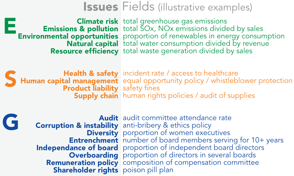
ESG data pertains to numerical fields that assess an entity’s (e.g., firm or country) performance with regard to one of the three thematic pillars: Environment, Social and Governance. Each pillar has several dimensions, also known as issues. The latter can even be further decomposed into sub-issues.
Raw numbers are simply fields (ex: CO2 emissions). Fields are processed or aggregated into synthetic scores at the issue and pillar level. These scores give a rough idea of the performance of the entity with respect to each pillar or issue.
NOTE: aggregation is much more complex than it seems (see below). Some fields are beneficial, others detrimental and others should be compared to industry standard. Moreover, aggregation is very complex in the presence of missing fields which happens all the time!
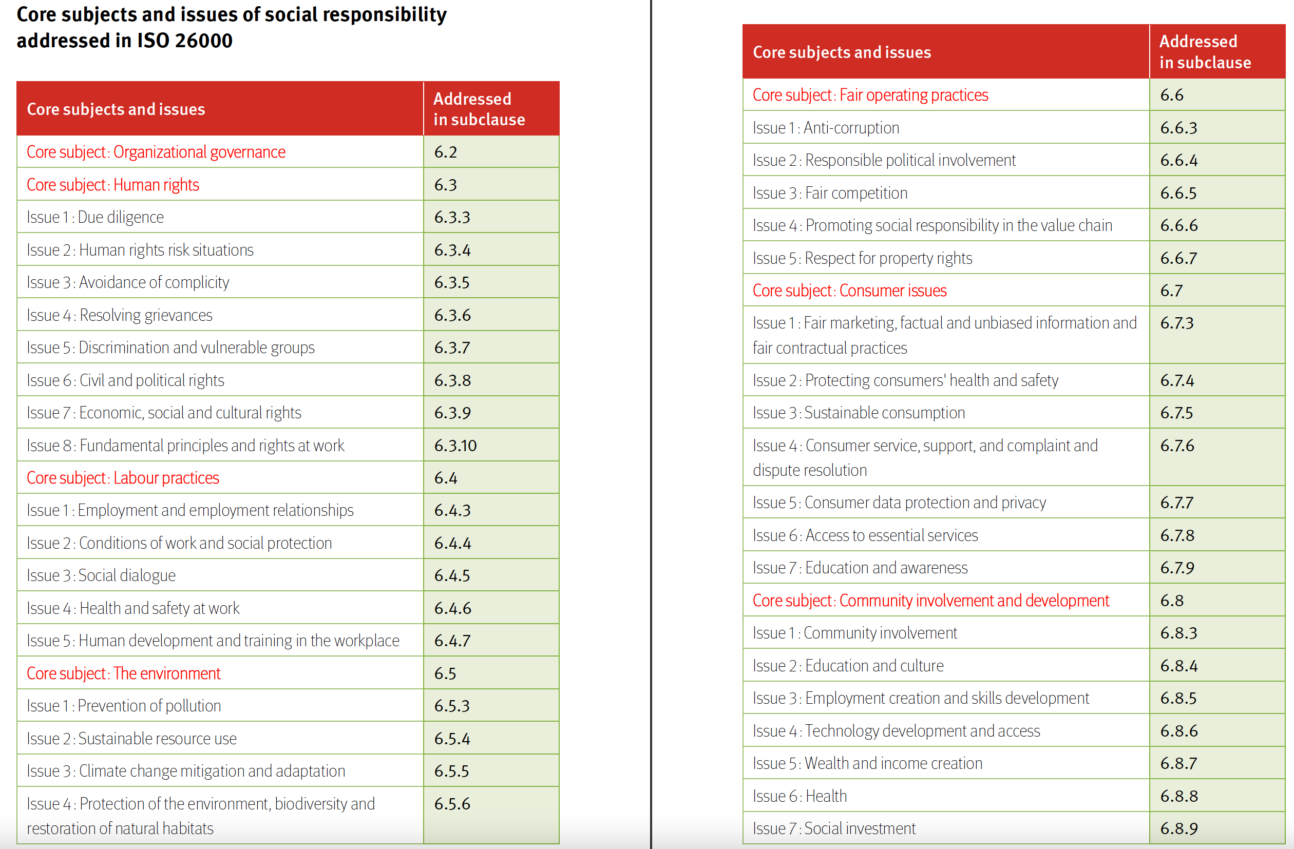
Another classification, from the ISO 26000 framework: it provides recommendations, but is not a certification.
Of course, as will be recalled multiple times, access to ESG data depends on firms’ will to accurately calculate figures and disclose them to the public. Because of the push for transparency, more and more firms are incentivized to do so. For instance, the CDP Project is an initiative that gathers data on carbon emissions of companies. The coverage of their dataset increases in time:
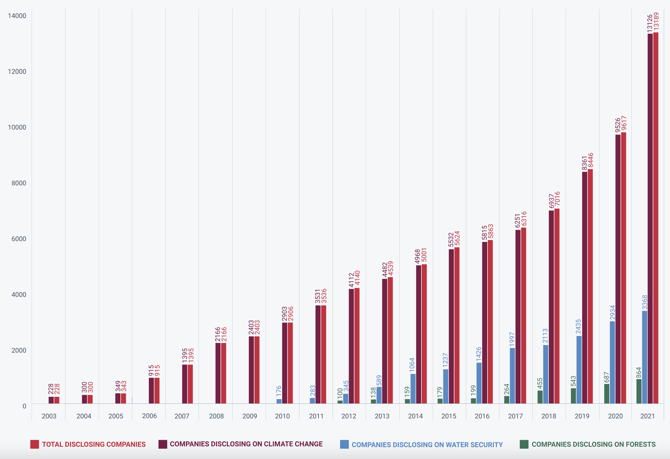
See also the CDP dashboard for more recent numbers.
Thanks to new regulations, this trend is poised to continue. In particular, the Net-Zero Data Public Utility seeks to provide a free platform with access to ESG-related fields for a large number of firms. Such initiatives will help standardize disclosure and hopefully increase transparency.
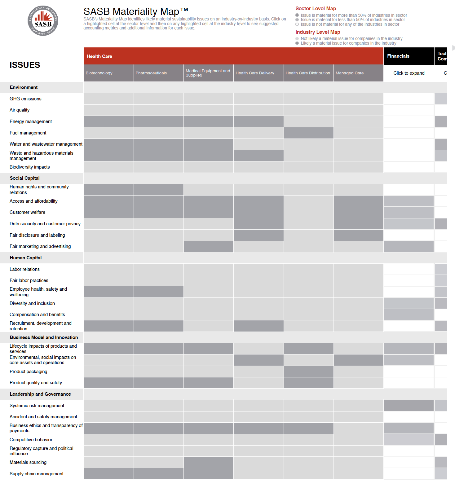
3.1.2 Materiality
An important concept in ESG fields is that of materiality. Basically, materiality refers to fields that matter for an organization’s business (in the sense: way of functioning). For instance:
- for a hospital, the ability to treat patients with equal care matters (S pillar);
- in a farm, reducing the use of pesticides is important (E pillar);
- in the printing industry, optimizing upstream & downstream paper recycling is crucial (E pillar). Basically this means printing on recycling paper & in turn recycling a maximum of paper waste.
Therefore material indicators depend very much on the way the entity works. Paper recycling is not a major issue in a farm - it is not material.
The SASB (Sustainability Accounting Standards Board) provides a mapping that helps assess materiality in ESG fields (http://sasb.s3-website-us-east-1.amazonaws.com/).
Originally, materiality came from the accounting world. Some accounting fields were deemed financially material if they were expected to have an effect on the financial performance of the firm. Thus, in the original definition, ESG materiality inherited this notion of financial impact, but for ESG fields. The effect that matters is ESG \(\rightarrow\) finances / corporate performance.
However, it is clear that this is narrow, from an ESG perspective. Indeed, in a modern context, the social & environmental consequences should also be examined. This is where double materiality kicks in (see diagram below, from the report entitled Guidelines on Reporting Climate-Related Information, by European Commission)
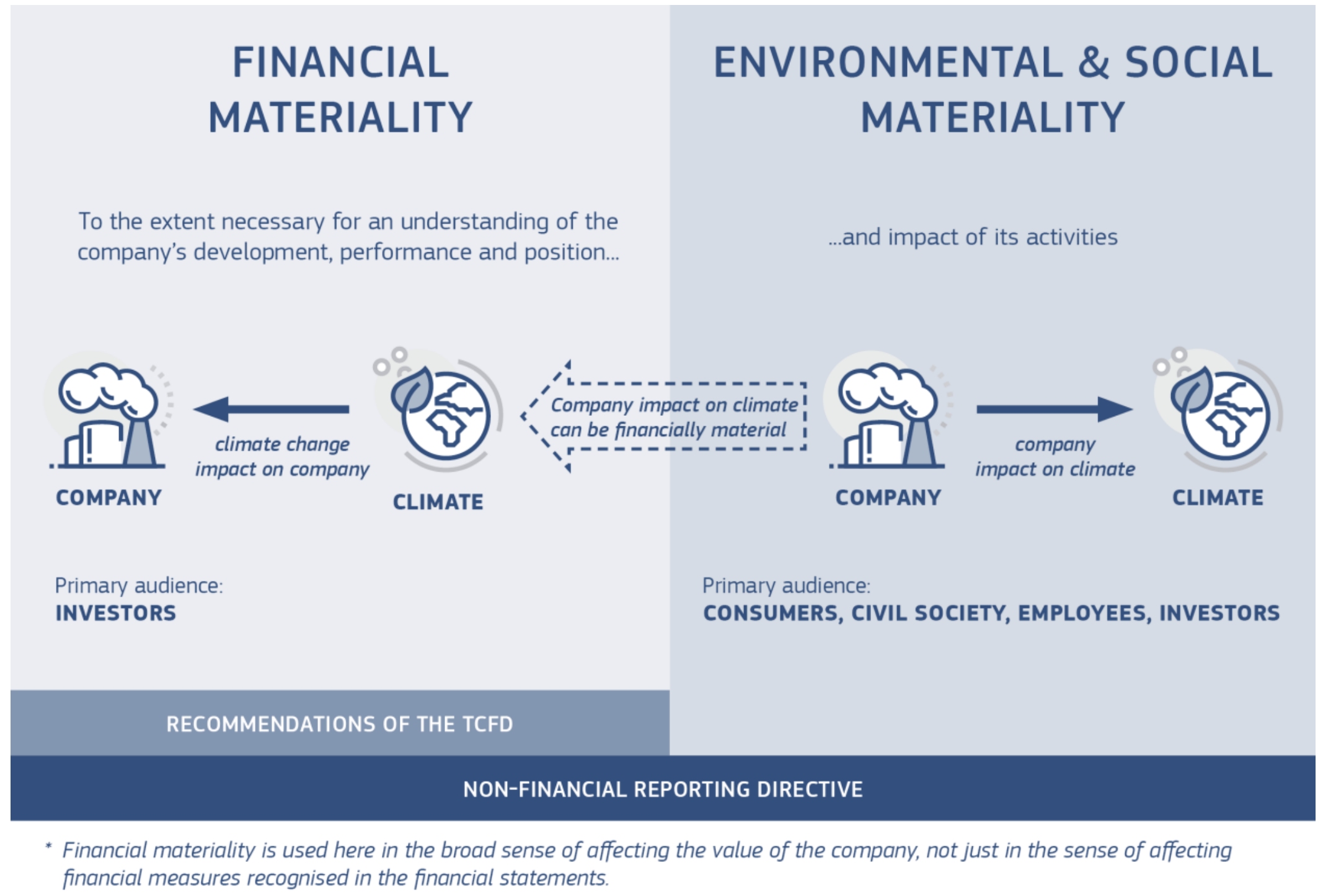
One way to interpret this is: ESG dimensions (climate incidents, social unrest) are likely to deteriorate business activity and hence financial performance. But reversely, business activity obviously has repercussions on the environment and social welfare (think: strikes in France!). The relationship goes both ways. However, some institutions like the International Sustainable Standards Board (ISSB), only advocate financial materiality…
In What information is relevant for sustainability reporting? The concept of materiality and the EU Corporate Sustainability Reporting Directive, from the Sustainable Finance Research Platform even advocate wider notions of materiality.
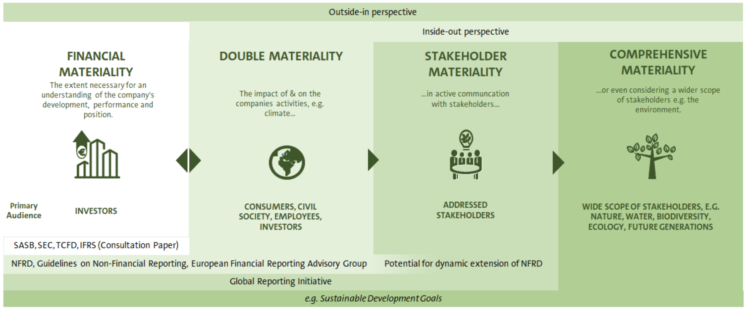
Stakeholders (clients, employees) are again put forward.
3.1.3 Greenwashing?
Strictly speaking, greenwashing relates to the marketing sphere. The Wikipedia definition is: a form of advertising or marketing spin in which green PR and green marketing are deceptively used to persuade the public that an organization’s products, aims and policies are environmentally friendly. One of the most common examples is H&M, with is clothing line “Conscious”, which misused the Higg Materials Sustainability Index.
It is possible that the term be “recycled” to attempts to artificially improve sustainable reporting in order for the firm to appear greener than it actually is. One adjacent issue is the labeling of “sustainable” financial products, like funds. In August 2021, the financial regulators in the US (Securities and Exchange Commission - SEC) and Germany (BaFin) revealed they were investigating DWS, a subsidiary of Deutsche Bank, and the second largest fund manager in Europe. In May 2022, DWS offices were raided by the German police. In 2020, DWS claimed to have 459B€ of green assets under management (funds incorporating ESG criteria for investment decisions). The figure sank to 115B€ in 2021…
This example shows that it has become very risky (and will become riskier) to dupe investors into buying wrongly labelled green funds. This is very beneficial for the industry - and maybe, at the end of the line, for the environment & society.
Lastly, though it’s not necessarily related, new terms have emerged:
- “greenwishing”: this refers to firms that publicly set very ambitious environmental targets, but fail to provide rigorous explanations on how they will achieve their goals. Cheap talk is not binding, but investors are not (always) fools either…
- “greenhushing”: (NOTE: the definition is not unambiguous!) this is either when a green company engages in some form of sustainability but refrains from communicating about it, OR when a brown company under-reports on purpose because its numbers are bad. Be careful: people can disagree on this one!
-
greenlighting: communicating excessively on a green feature of a product. Possibly in order to take attention away from browner product lines.
- see also: greenrinsing, greenshifting, etc.
3.2 The playing field
3.2.1 Landscape of providers
First, we present the players: the rating agencies.
A bit of history. For a relatively long period of time (until 2015-2020), the traditional data providers (Bloomberg, Thomson-Reuters) and agencies (Moodys, S&P) did not care much about sustainability scores and ratings. Thus, it was turf of a few specialized actors, like KLD and Vigeo Eiris. Then, the field started consolidating (see below) and big players acquired the smaller specialists.
However, this raises new concerns of conflicts of interests. For instance, what happens when Trucost (which belong to S&P Global) must rate IHS Markit or S&P Dow Jones Indices, which are all subsidiaries of S&P Global?
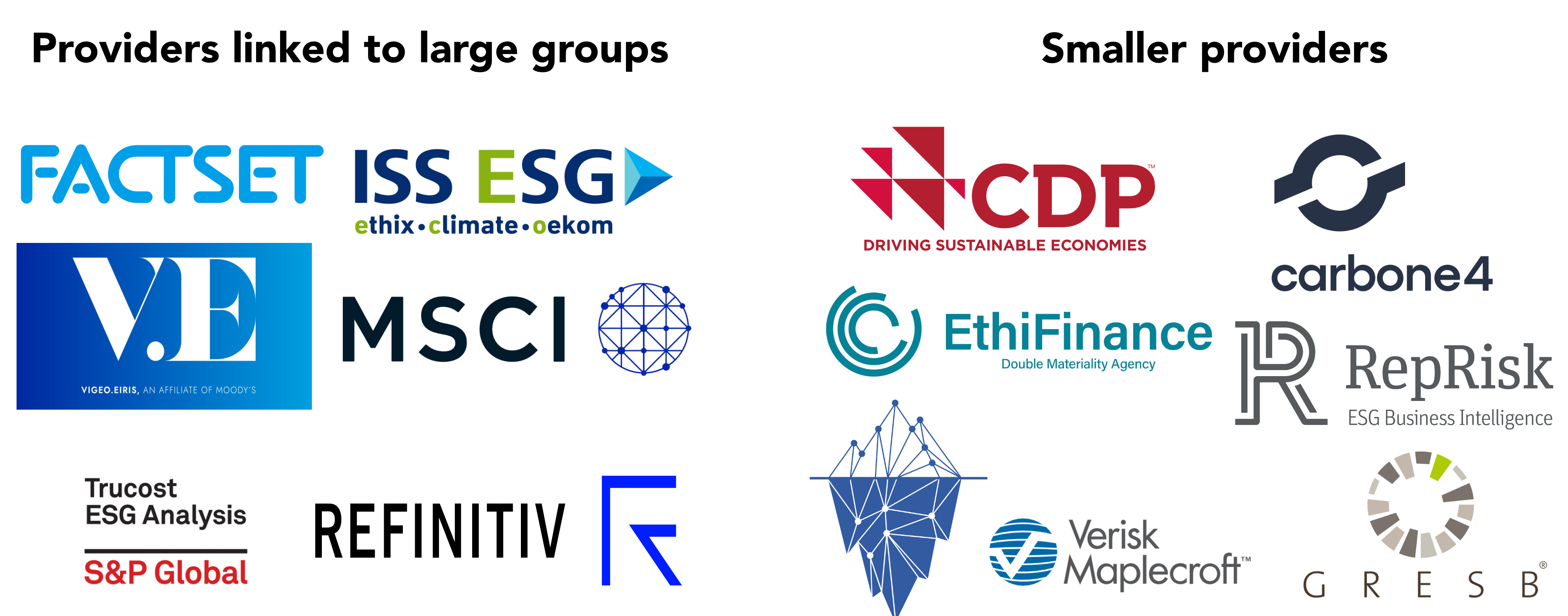
A table with some links below:
| Big players | Smaller providers |
|---|---|
| Factset (with TruValue Labs) | Carbon Disclosure Project |
| ISS (Deutsche Börse) | Carbon4 Finance |
| FTSE Russel (London Stock Exchange) | Covalence |
| Moody’s (with Vigeo Eiris) | EthiFinance |
| MSCI (with Riskmetrics) | Global ESG Benchmark for Real Assets |
| Refinitiv (London Stock Exchange) | Iceberg Datalab |
| Sustainalytics (Morningstar) | Maplecroft |
| TruCost (S&P) | RepRisk |
Other players include CSRHUB, Equileap (for gender parity), Ethos ESG, Inrate
3.2.2 Consolidation
NOTE: The field has consolidated, some firms diluted in larger groups: 427 (Moody’s), Truvalue Labs (Factset), Oekom (ISS), RiskMetrics-KLD-Carbon Delta (MSCI), Solaron (Sustainalytics).
For a detailed view, we refer to the report Provision of non-financial data: mapping of stakeholders, products and services by Anne Demartini for the French AMF (autorité des marchés financiers).
| Year | Month | Target | Acquirer |
|---|---|---|---|
| 2009 | February | Innovest (US) | Riskmetrics (US) |
| September | Merger of Sustainalytics (Netherlands) and Jantzi Research Inc. (CND) | ||
| November | Asset 4 (Switzerland) | Thomson Reuters (US) | |
| KLD (US) | Riskmetrics (US) | ||
| December | New Energy Finance (UK) | Bloomberg (US) | |
| 2010 | March | Riskmetrics (US) | MSCI (US) |
| 2012 | June | Responsible Research (Singapore) | Sustainalytics (Netherlands) |
| 2014 | June | GMI Rating (US) | MSCI (US) |
| July | zRating (Switzerland) | ||
| 2015 | September | Ethix SRI Advisors (Denmark) | ISS (US) |
| ESG Analytics (Switzerland) | Sustainalytics (Netherlands) | ||
| October | Fusion Vigeo (FR) / Eiris (UK) | ||
| 2016 | October | Trucost (UK) | S&P Global (US) |
| 2017 | June | South Pole / Investment Climate Data Division (Switzerland) | ISS (US) |
| July | Sustainalytics (Netherlands) – acquisition of a 40% stake | Morningstar (US) | |
| 2018 | March | Oekom (Germany) | ISS (US) |
| Solaron (India) | Sustainalytics (Netherlands) | ||
| 2019 | January | GES International (Sweden) | Sustainalytics (Netherlands) |
| March | Vigeo-Eiris (FR) | Moody’s Corp (US) | |
| June | Beyond Ratings (FR) | London Stock Exchange (UK) | |
| July | Four Twenty Seven (US) | Moody’s Corp (US) | |
| August | Refinitiv (formerly Thomson Reuters, US) | London Stock Exchange (UK) | |
| September | Carbon Delta (Switzerland) | MSCI (US) | |
| October | Ethical Corp (US) | Thomson Reuters (US) | |
| November | Robecosam AG-ESG Ratings Business (Switzerland) | S&P Global (US) | |
| 2020 | January | Ecovadis (FR)- Acquisition on a non-controlling interest | CVC Growth Partners (US) |
| April | Sustainalytics (Netherlands) – 100% stake | Morningstar (US) | |
| October | TrueValueLab (US) | Factset (US) | |
| November | ISS (US) | Deutsche Börse | |
| Merger of IHS Markit (US) and S&P Global (US) |
3.2.3 A booming industry
The increasing demand for ESG data incites providers to spend more on the research & acquisition side:
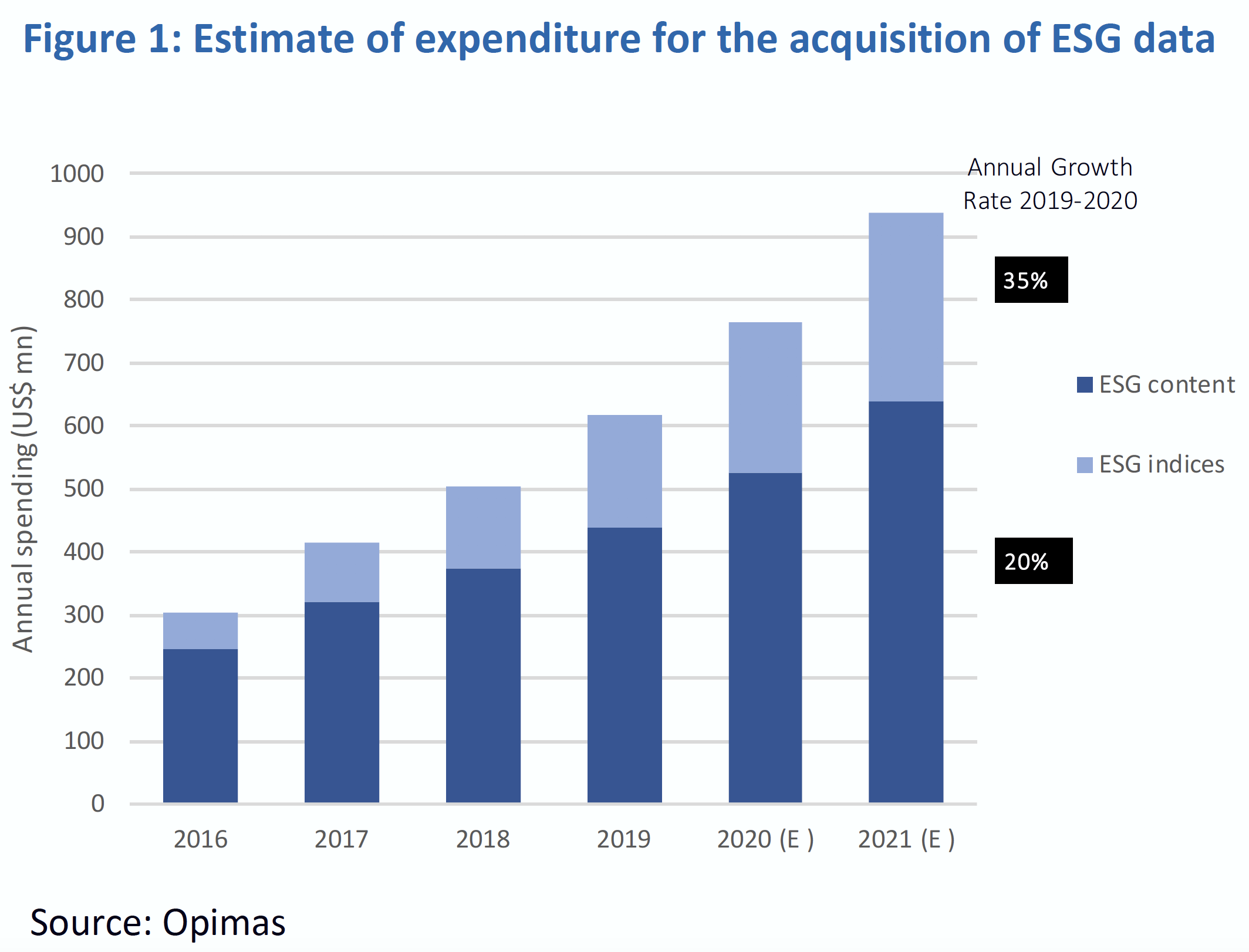
One reason is that investors want information that is reliable, i.e., that accurately reflects the policies of firms. But this is very costly. The main explanation for this is that, as of 2022, no coercive framework forces corporations to report precise non-financial metrics, as is the case for standard accounting via balance sheets and income and cash-flow statements (EBIT, Total assets, investments, revenue, etc.).
3.2.4 Diversity in raters
We refer here to the insightful report Rate the raters: ESG ratings at crossroads. This report compiles results from a survey carried out by the Sustainability institute. A few enlightening graphs below, especially with regard to quality perception (by respondents).
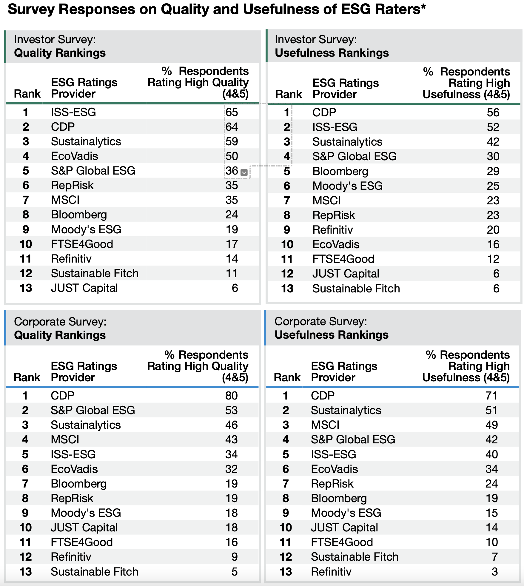
The CDP makes it to the top 2 spots on all criteria.
Some differences between raters:
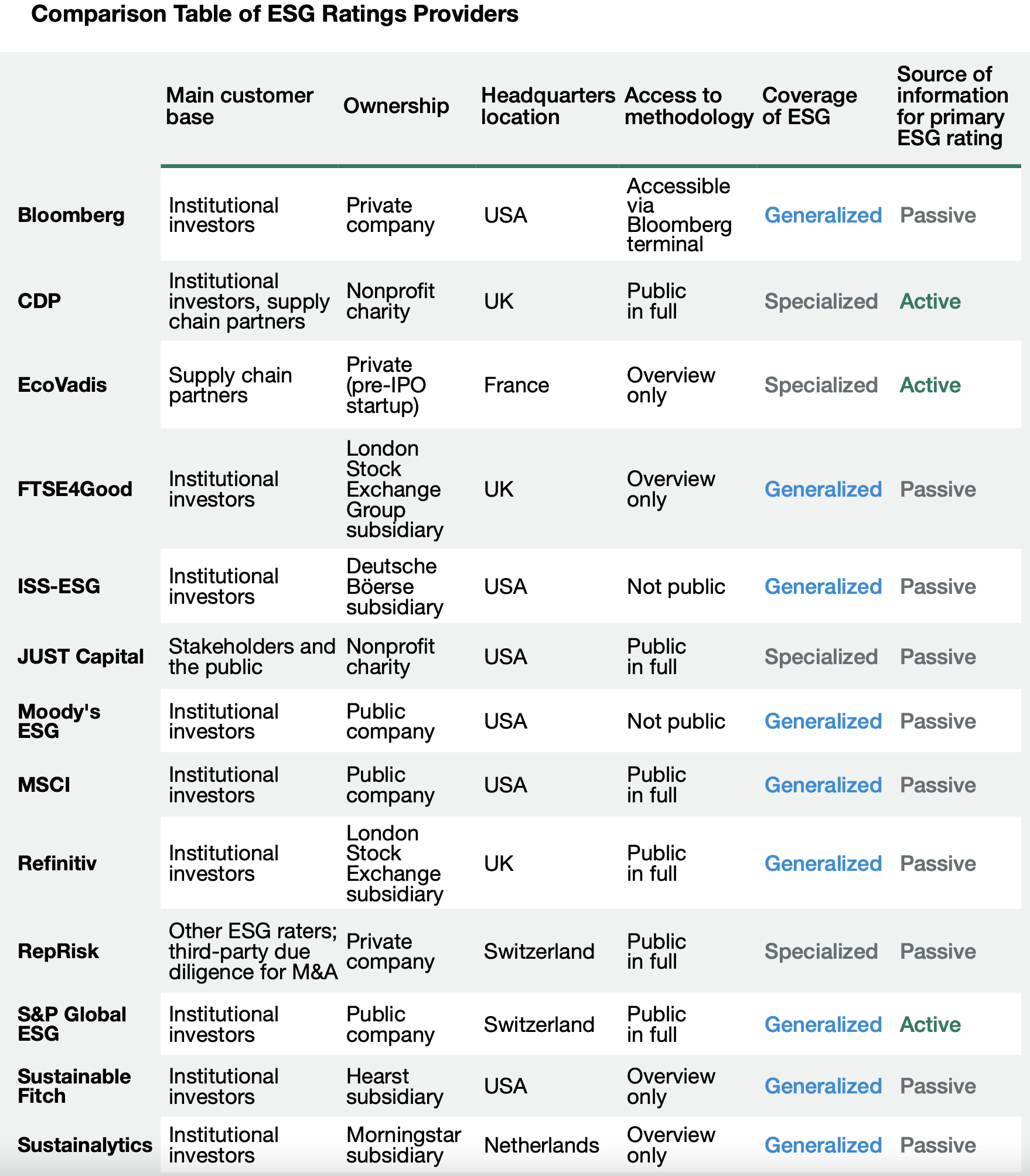
NOTE: active means that in order to be rated, companies need to respond to lengthy questionnaires.
Also: the CDP only focused on carbon, water and forests (hence, the environment): thus it is specialized. Generalized raters take into account all three pillars.
3.3 How are ESG data collected or constructed?
The raw material that is used to craft firm-specific metrics is of two types:
-
internal: the rater trusts documents disclosed by the company (e.g.: in annual reports, especially those dedicated to sustainability which are mostly compiled by large firms).
- external: the rater gathers data from outside the firm, such as: whistleblowers, social media, digital surveys (ex: synthesio), etc.; or try to estimate values from trustworthy fields, like accounting fields (which are regulated by norms & standards).
In some cases, there might not be the choice, as some fields are not provided by companies. Typically, each firm chooses which item it wishes to communicate in its (often CSR-ESG-dedicated) annual report. This is a major issue for providers because the lack of norm can make it hard to compare figures (e.g., GHG vs carbon emissions).
3.3.1 European regulation
Thus, the topic of non-financial (or sustainability) reporting is crucial. In Europe, under the original (chronologically) Non-Financial Reporting Directive (NFRD), large firms (>500 employees) with public interest must already provide basic ESG-related information. But fields and metrics were not standardized, and companies were free with respect to the methodology. This made comparisons impossible, so that data was not optimally useful.
The objective, via the Corporate Sustainability Reporting Directive (CSRD), is to extend this to all large companies. Listed small and medium-sized enterprises (SMEs) have until 2026 to comply. Non-European companies with substantial activity in Europe are also involved.
Basically, this means corporation will have to provide much more sustainability-related information. Just like for financial disclosures, it will be warranted (e.g., by assurance providers) and possibly audited.
Also, the reform puts forward the EU Taxonomy, which is a set of classifications that determines which activities are sustainable and which are not.
Finally, for the financial sector, the European Supervisory Authorities (“ESAs”) have also validated the regulatory technical standards (RTSs) after crafting the Sustainable Finance Disclosure Regulation (SFDR). This will allow investors to better understand the goals and purposes of financial instruments, such as funds for instance. The text proposes a classification of funds and mandates into three categories, which are defined in articles:
-
Article 6: investment vehicles that do not integrate any kind of sustainability in their construction process. They are not forbidden but must clearly be labelled as non-sustainable.
-
Article 8: for environmental and socially promoting funds. Also known as light green funds: funds which promotes, among other characteristics, environmental or social characteristics, or a combination of those characteristics, provided that the companies in which the investments are made follow good governance practices. The fund manager must use the sustainability indicators (see below) actively in the allocation process.
- Article 9: products targeting sustainable investments. Here, greenness is the objective, it’s not just a tool. Typically, a fund that focuses on GHG emission reduction can be Article 9, but in this case, it must thoroughly prove how it will achieve its goal, especially in comparisons of benchmarks.
The latter two are of course more constraining, as they require active reporting on the following dimensions: summary of the fund, monitoring of synthetic ESG characteristics, investment strategy, proportion of ESG vs non-ESG assets.
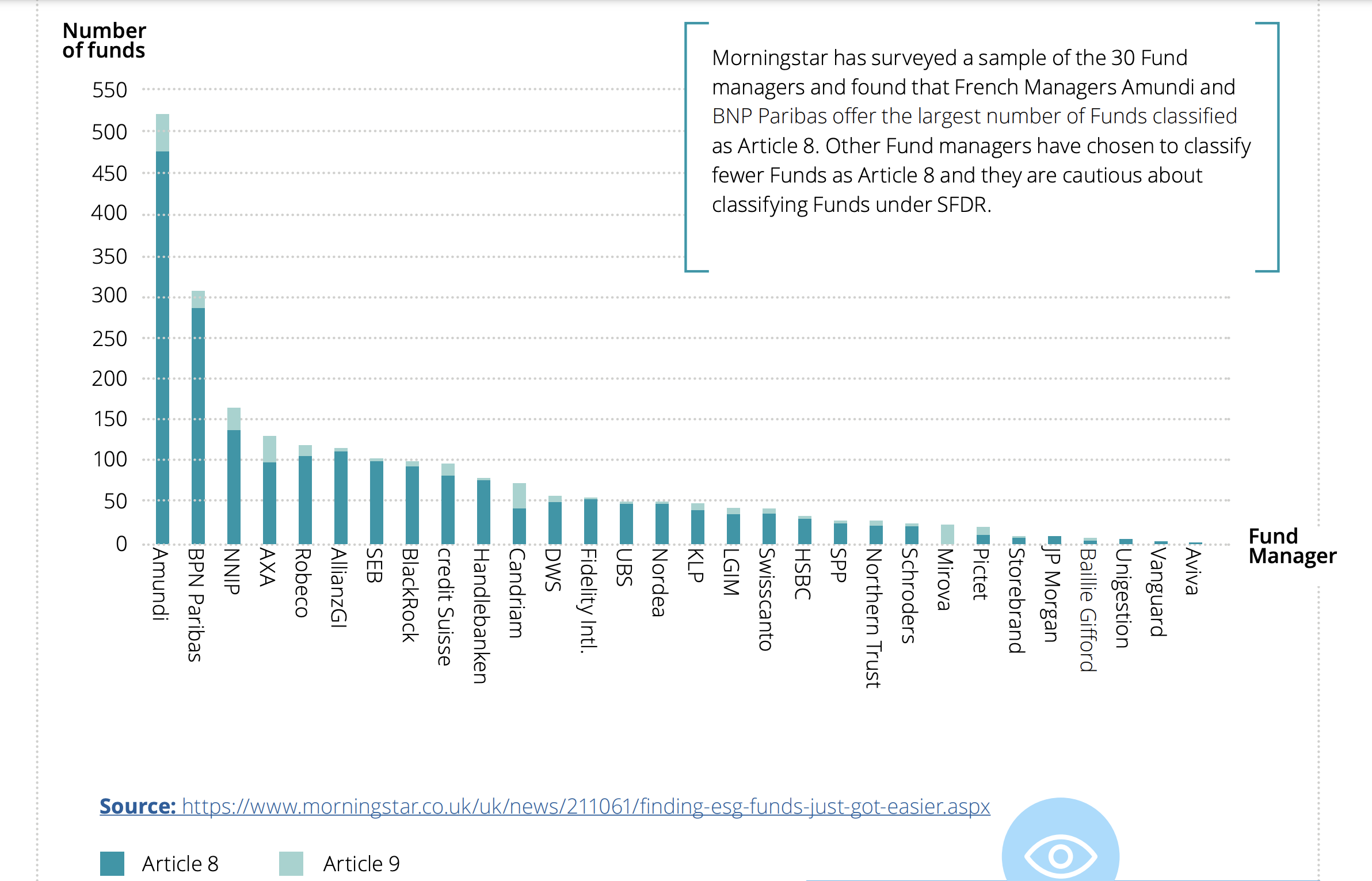
Morningstar now tracks A8 and A9 funds (& flows) actively.
A snapshot of the amount of green funds under SFDR (source: Deloitte, based on Morningstar data):
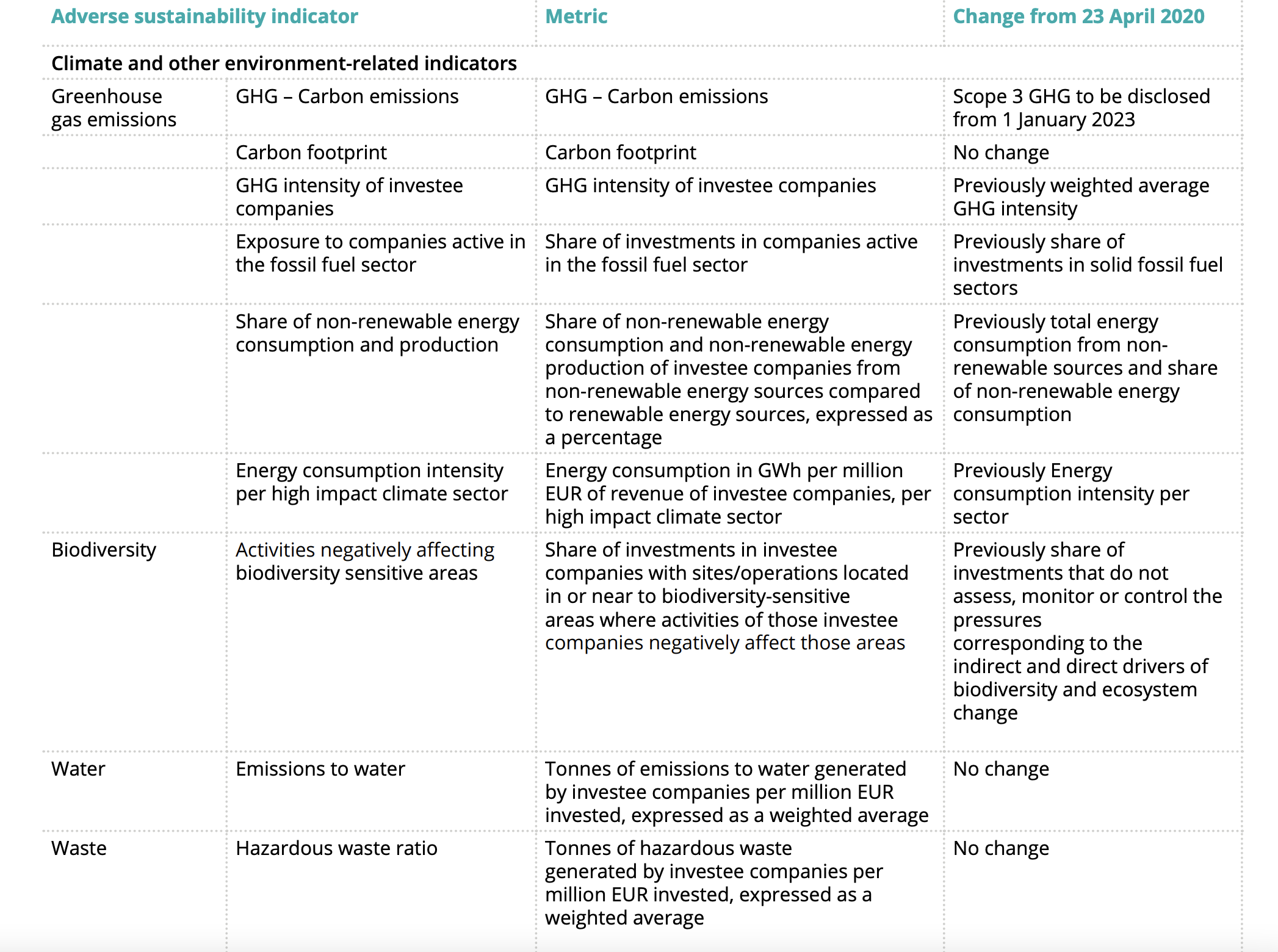
Examples of compulsory environmental fields, a.k.a., PASI “principal adverse sustainability indicators” (source: Deloitte):
3.3.2 A dive into corporate documents
Let’s first have a look at annual reports. Take Total Energies for instance. (All major firms have environment-related disclosure, see Apple for instance).
From the 2020 Universal Registration Document, we extract:
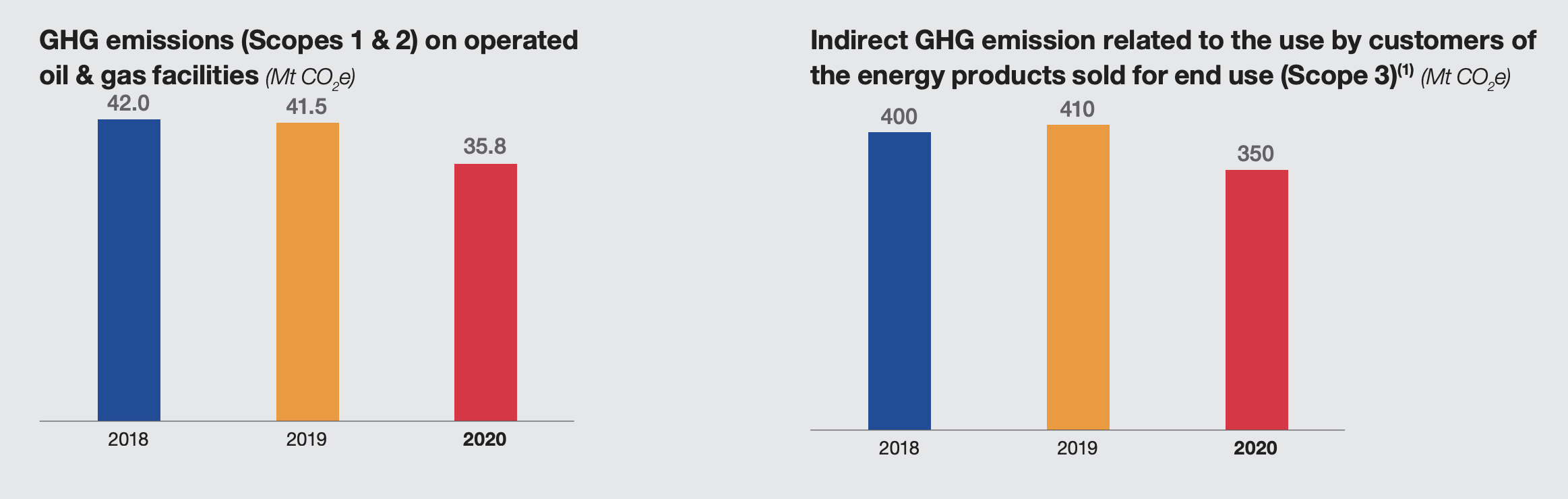
NOTE: there are more than 200 mentions of CO2 in the reports. Finding the same graph in the 2021 report is hard. You have to go page 304 (out of 664!) to get precise figures:
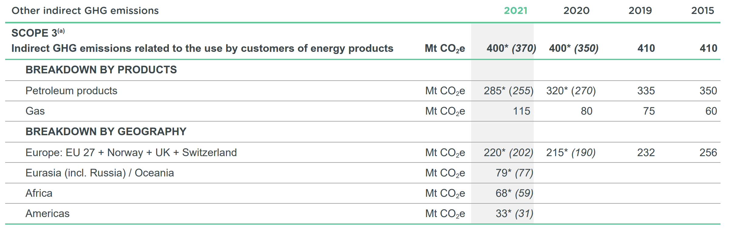
This is a typical illustration of why gathering data from reports is incredibly time-consuming because of formatting inconsistencies from one report to the next one. Training a bot or a supervised algorithm to do the work is very hard. Best results are probably reached by fetching the numbers manually - but this makes many numbers, for many companies, each quarter or year. In turn, this daunting task augments the risk of human failure.
In the 2021 report, Total mentions its intent to “Reduce the indirect emissions related to its products (Scope 3), together with society – i.e., its customers, its suppliers, its partners and public authorities – by helping to transform its customers’ energy demand.” Tying its goals with society is a prudent commitment… basically: they will do their best, but not alone. That can be referred to as greenwishing.
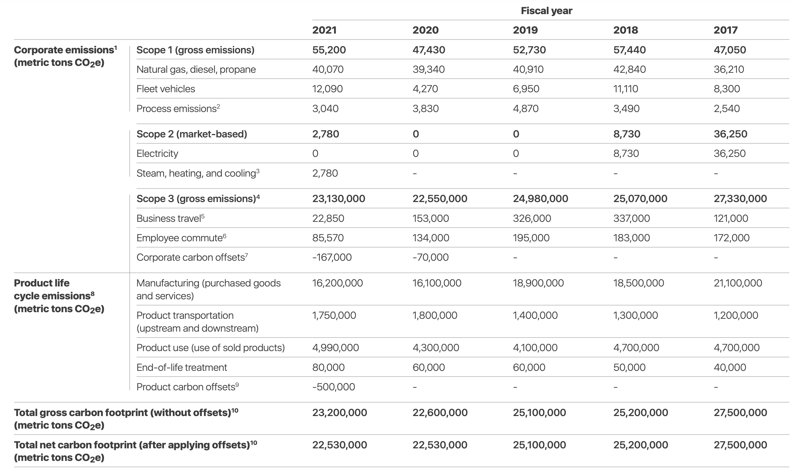
Naturally, each firm is free to write its report more or less in its chosen terms - and difference arise from country to country. Take Apple: the company even had an ESG page/platform: https://investor.apple.com/esg/default.aspx which is no longer active (so long for ESG; the page in 2024 is: https://www.apple.com/environment/#reports-product). It has a dedicated Environmental Progress Report and, more generally, an ESG report as well and both are updated annually. In the latter, the social pillar is a lot focused on gender and race - for equality, diversity & inclusion purposes. In the former (& the latter too), we get a good overview of emissions:
FUN FACT: in corporate reports, companies often mention “targets” (e.g., with respect to 5-20 years in the future) more than actual figures… This is a well known trick (also works for governments) because long term goals are often not implemented by those who decide and fix them. Pious wishes! Greenwishing again.
3.3.3 Aggregating fields
ESG is by essence multi-dimensional - if only because there are at least the 3 pillars! In practice, there are many issues that one would want to include into the analysis, but in the end, we often need one synthetic score that captures all the information. Thus, we have to aggregate figures, and this is hard - for two reasons:
- First, there is the diversity in fields. For instance, some are numerical, some categorical (e.g., binary: does the firm have an ESG officer, or a anti-child labor policy?). Moreover, sometimes, some numerical fields are greener if they are high (% of recycling), sometimes it’s better when they are small (emissions). Even worse, there are some fields for which average values are preferred. For instance: CEO tenure. Typically, short tenure is not great (less experience in the firm), but long tenure is also not a good signal (firms need fresh new ideas and CEO rotation is healthy, up to a point). Thus, a huge amount of coding, standardizing and weighting is required. First, all fields must be:
-
digitized (translated into numbers - this may require one-hot encoding in rare cases),
-
ordered (so that high values are preferred - this may mean being close to an (industry?) average value, as for CEO tenure) and
- standardized, so that they all have the same (or similar) scale
- Then, it’s all a matter of weighting, and this will depend on preferences. For instance, given synthetic scores for each pillar, it is customary to take the simple average of the three (E+S+G)/3, but it is entirely possible to give more weight to one pillar in particular (1/2 + 1/4 + 1/4 for instance).
- The second issue is missing data, a real pain in the discipline. One partial solution is simply to include a coverage score, wherein the amount of data disclosed by the company is a field of its own - and can have a substantial impact on the overall score. The other alternative is imputation, whereby we attribute a “fake” (or guessed) score to the company for a given field. There are many ways to perform imputation, depending on preferences and beliefs. The most conservative option is to give the firm the worst possible score, in order to strongly penalize the corporations that refuse to disclose (but sometimes it’s also a question of lack of resource to do so… large firms clearly have an advantage here). A common option is to give an average (or median) value - either over all firms, or over all the firms of the same sector. Finally, it is also possible to resort to exposure estimation, as with the carbon beta.
In the end, the methodology that rating agencies use to compute synthetic scores is often considered as intellectual property, though some of them are quite transparent about how they proceed (white papers are sometimes available). But in the end, it is the gathering of granular data that is the most time-consuming. Aggregation is a matter of many choices, but is easily automated.
3.4 Exploring a dataset on US corporations
3.4.1 Introduction
ESG data that is:
- free,
- updated and with time-series ,
- available for many companies
is rare, if it exists at all. Yahoo Finance used to be an exception when providing Sustainalytics’ ESG Risk Ratings. However, it is no longer disclosing this kind of information and at the time (until 2025), only the current score was made available (not the full history). Moreover, scrapping Yahoo takes a lot of time (hours & hours), even with automated scripts.
Another interesting source is the Science Based Targets, which provides an up to date dashboard. Again, there is only static data, and the number of firms is about 4200+ at the end of 2023.
This is where ESG data vendors come in handy. Their databases are useful, but quite expensive.
We extracted data from two traditional vendors, which are anonymized. We make important comments about the dataset:
- data from Provider A is sampled monthly, while Provider B data is sampled yearly of each firm, though points may change quarterly, depending on which firm is covered.
- Data starts in Dec. 2005 for Provider A, and in 2001 for Provider B.
- Market_Cap is absent from Provider B, and E, S and G pillars are absent from Provider A.
- Missing points were imputed: when an absent field is preceded by a number, the latter replaces the former.
- We use ESG_Metric for both providers, but it is a score for Provider B, and in contrast a risk score for Provider A. Hence, in the latter, a high score is bad. ESG data for Provider A starts very late (2021).
- Scopes for Provider A refer to total GHG (in thousands of metric tons of carbon dioxide equivalent (kmtCO2e)), while for Provider B, they are CO2 emissions (originally in mtCO2e, but manually changed to kmtCO2e). In some cases, the distinction may be subtle, as CO2 is the major source of GHG.
- Many fields are missing. For instance, the closing price of American Airlines (AAL) is only available from 2013 onwards. This comes from the merger with US Airways. In many other cases, e.g., for Scope data, the values are simply not known (e.g., not disclosed by firms).
The data is available on Github, in R format (.RData) as well as in Excel (.xlsx) format.
\(\rightarrow\) It is meant to play with, and for pedagogical purposes only!
load("ESG_data.RData")  # This is to import the file (in the present directory)
ESG_data |> tail(10) # This is to see the last 10 rows of the data| source | date | instrument | name | sector | close | market_cap | profit_margin | esg_metric | scope_1 | scope_2 | scope_3 |
|---|---|---|---|---|---|---|---|---|---|---|---|
| Provider_B | 2023-06-30 | YUM | Yum! Brands Inc | Accommodation and Food Services | 138.55 | 36078581877 | 48.33 | 79.98 | 42.92 | 100.48 | 29578.6 |
| Provider_B | 2023-07-31 | YUM | Yum! Brands Inc | Accommodation and Food Services | 137.67 | 36078581877 | 48.33 | 79.98 | 42.92 | 100.48 | 29578.6 |
| Provider_B | 2023-08-31 | YUM | Yum! Brands Inc | Accommodation and Food Services | 129.38 | 36078581877 | 48.33 | 79.98 | 42.92 | 100.48 | 29578.6 |
| Provider_B | 2023-09-30 | YUM | Yum! Brands Inc | Accommodation and Food Services | 124.94 | 36078581877 | 48.33 | 79.98 | 42.92 | 100.48 | 29578.6 |
| Provider_B | 2023-10-31 | YUM | Yum! Brands Inc | Accommodation and Food Services | 120.86 | 36078581877 | 48.33 | 79.98 | 42.92 | 100.48 | 29578.6 |
| Provider_B | 2023-11-30 | YUM | Yum! Brands Inc | Accommodation and Food Services | 125.55 | 36078581877 | 48.33 | 79.98 | 42.92 | 100.48 | 29578.6 |
| Provider_B | 2023-12-31 | YUM | Yum! Brands Inc | Accommodation and Food Services | 130.66 | 36612405975 | 49.41 | 79.98 | 42.92 | 100.48 | 29578.6 |
| Provider_B | 2024-01-31 | YUM | Yum! Brands Inc | Accommodation and Food Services | 129.49 | 36612405975 | 49.41 | 79.98 | 42.92 | 100.48 | 29578.6 |
| Provider_B | 2024-02-29 | YUM | Yum! Brands Inc | Accommodation and Food Services | 138.42 | 36612405975 | 49.41 | NA | NA | NA | NA |
| Provider_B | 2024-03-31 | YUM | Yum! Brands Inc | Accommodation and Food Services | 138.65 | 36612405975 | 49.41 | NA | NA | NA | NA |
3.4.2 Coverage and missing data
To evaluate the state of missing data, we resort to a dedicated package called visdat - it needs to be installed to be used.
ESG metrics are quite empty (grey zones), with emissions also sometimes missing.
Let us now look at coverage. We define coverage as the number of firms for which a given field is provided.
For instance, below, we look at the ESG metric.
ESG_data |>
  filter(year(date) > 2002, year(date) < 2024) |>
  group_by(source, date) |>
  summarize(n = sum(is.finite(esg_metric))) |>
  ggplot(aes(x = date, y = n, color = source)) + geom_line() +
  theme_bw()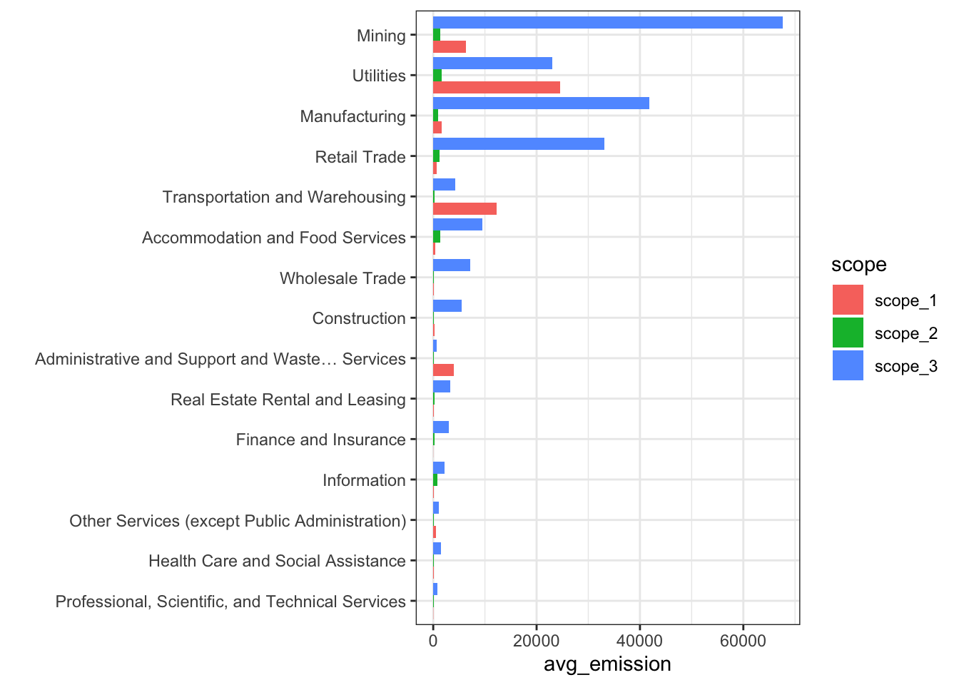
Unfortunately, ESG data for Provider A is only available very lately (change in their offering 👎 😞). It seems they decided to change their approach (business model) and require additional licensing for sustainable fields…
For Scope 1 emissions, more data is available.
ESG_data |>
  filter(year(date) > 2002, year(date) < 2024) |>
  group_by(source, date) |>
  summarize(n = sum(is.finite(scope_1))) |>
  ggplot(aes(x = date, y = n, color = source)) + geom_line() +
  theme_bw() +
  scale_color_manual(values = c("#EE9911", "#1199EE"))
3.4.3 Descriptive statistics
Most people/students hate the word “statistics”. Yet, statistics offer huge amounts of very useful tools, especially to rapidly understand & characterize data.
Let us take a first look at the distribution (across all years) of Scope 1 emissions taken from the dataset of Provider 1.
ESG_data |>
  filter(year(date) > 2002, year(date) < 2024) |>
  filter(source == "Provider_A") |>
  ggplot(aes(x = scope_1)) + geom_histogram()
We see that the tail of the distribution is “fat”, meaning that there are observations (firms), which have huge Scope 1 emissions (> 100,000 ktCO2e). Nevertheless, a large majority of firms have emissions < 20,000 ktCO2e.
In order to have a plot that is easier to exploit, it is possible to use a logarithmic scale for the x-axis.
Let us try this for Scope 3 emissions.
ESG_data |>
  filter(source == "Provider_A") |>
  ggplot(aes(x = scope_3)) + geom_histogram(fill = "#2266EE", alpha = 0.7) +
  scale_x_log10() + theme_bw() + ylab("") +
  xlab("Scope 3 emissions in ktCO2e")
In the above graph, we see the scale goes even further: one million to the right!
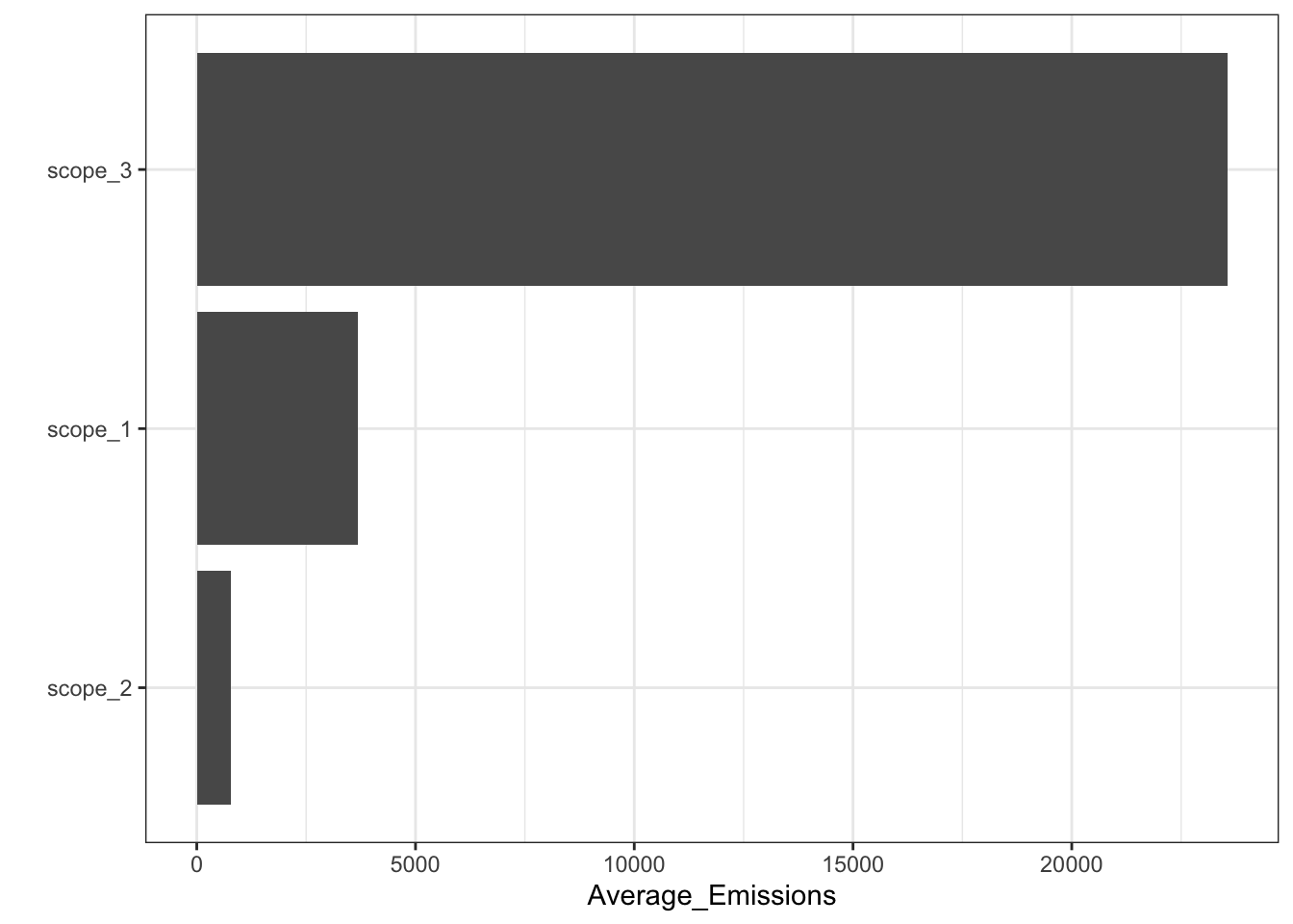
One important question is the relative importance of scopes.
Below, we select the observations for which we have all 3 scopes, compute average values for each firm and compare the average of the 3 scopes.
ESG_data |>
  filter(is.finite(scope_1 + scope_2 + scope_3),
         source == "Provider_A") |>
  summarise(scope_1 = mean(scope_1),
            scope_2 = mean(scope_2),
            scope_3 = mean(scope_3)) |>
  pivot_longer(cols = everything(),
               names_to = "Scope",
               values_to = "Average_Emissions") |>
  ggplot(aes(x = Average_Emissions, y = reorder(Scope, Average_Emissions))) + geom_col() +
  ylab("") + theme_bw()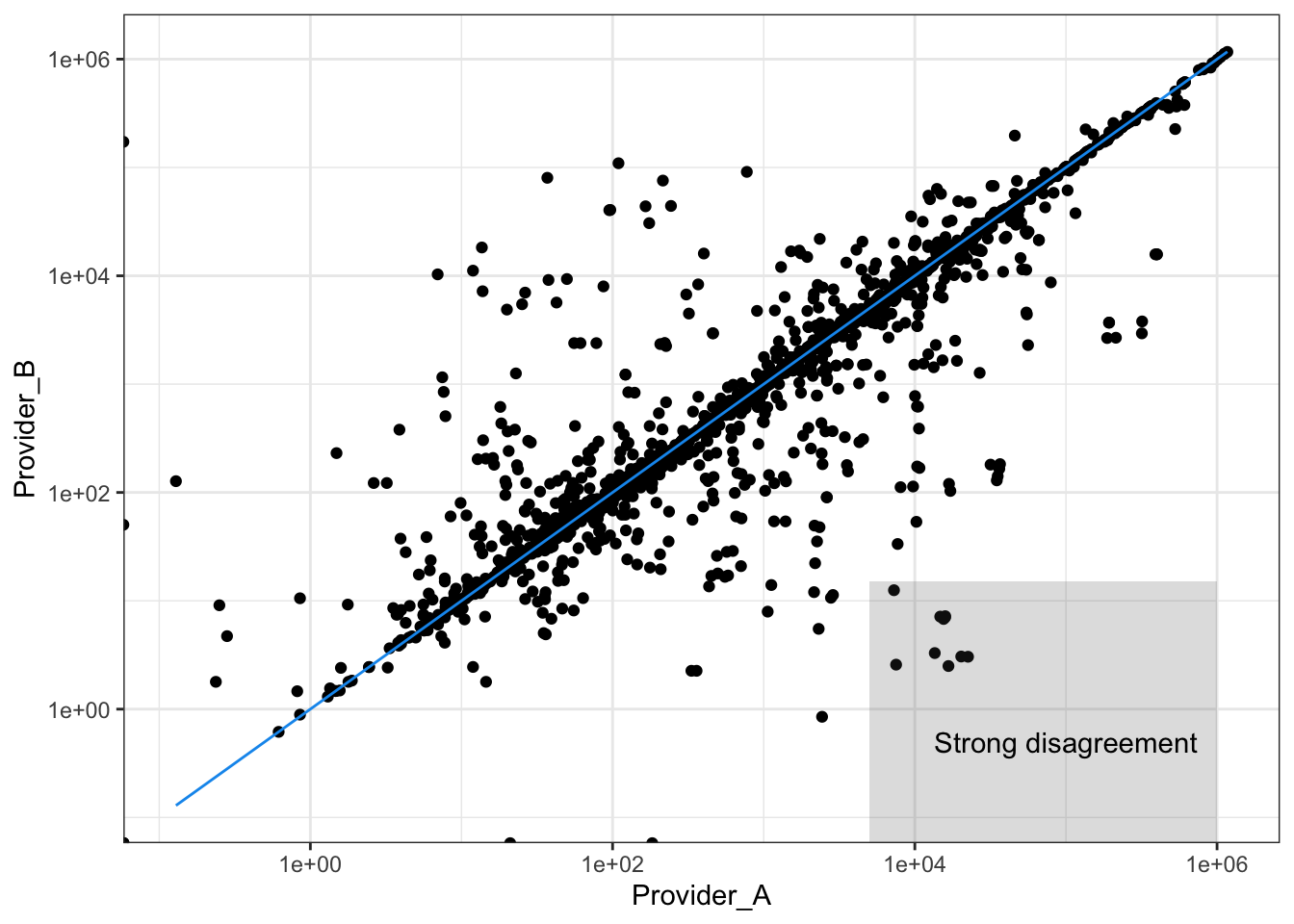
In the dataset, we have access to industry codes. Let’s have a look at what happens if we group by industry.
ESG_data |>
  filter(is.finite(scope_1 + scope_2 + scope_3),
         source == "Provider_A") |>
  pivot_longer(scope_1:scope_3, names_to = "scope", values_to = "value") |>
  group_by(sector, scope) |>
  summarise(avg_emission = mean(value)) |>
  ggplot(aes(y = reorder(sector, avg_emission), x = avg_emission, fill = scope)) +
geom_col(position = "dodge") + theme_bw() + ylab("") 
Now, there is an important issue with Scope 3 emissions: they are very hard to assess
Some companies have internal models to evaluate them, but the methodology is often opaque, as (again!) there is no regulatory framework that sets rules (e.g., formulae for each sector/industry - see below).
Some third party agencies have decided to create their own methodologies, based on accounting figures and industry standards in terms of business models.
Out of curiosity: who are the biggest polluters?
ESG_data |>
  filter(year(date) > 2002, year(date) < 2024) |>
  filter(source == "Provider_A", date > "2022-06-01") |>
  group_by(name) |>
  summarise(scope_3 = mean(scope_3, na.rm = T)) |>
  arrange(desc(scope_3)) |>
head(7) # Just extracting the top 19...| name | scope_3 |
|---|---|
| Cummins Inc | 1137784.7 |
| Caterpillar Inc | 604157.9 |
| Chevron Corp | 602684.2 |
| Emerson Electric Co | 597210.3 |
| Marathon Petroleum Corp | 455684.2 |
| General Electric Co | 410530.0 |
| Hartford Financial Services Group Inc | 374386.5 |
ESG_data |>
  filter(year(date) > 2002, year(date) < 2024) |>
  filter(source == "Provider_A", date > "2022-06-01") |>
  group_by(name) |>
  summarise(scope_1 = mean(scope_1, na.rm = T)) |>
  arrange(desc(scope_1)) |>
head(7) # Just extracting the top 19...| name | scope_1 |
|---|---|
| Southern Co | 83987.32 |
| Duke Energy Corp | 78505.26 |
| Chevron Corp | 54473.68 |
| American Electric Power Company Inc | 53053.04 |
| Nextera Energy Inc | 42376.78 |
| AES Corp | 40266.19 |
| Entergy Corp | 38026.32 |
3.4.4 ESG disagreement
3.4.4.1 In the literature
There is now abundant evidence that depending on your ESG data provider, your results/performance may change drastically.
Below, we cite a few papers that deal & have documented this effect. We point to the SSRN versions of the papers, as they are publicly available.
-
Dimson, Marsh, Staunton (2020),
-
Avramov, Cheng, Lioui & Tarelli (2021)
-
Gibson, Krueger & Schmidt (2021) &
- Berg, Kolbel, Rigobon (2022)
For instance, in the latter, the authors compute the correlation between ratings from 6 providers (see below). Some raters seem to somewhat agree with a few peers, and strongly disagree with others.
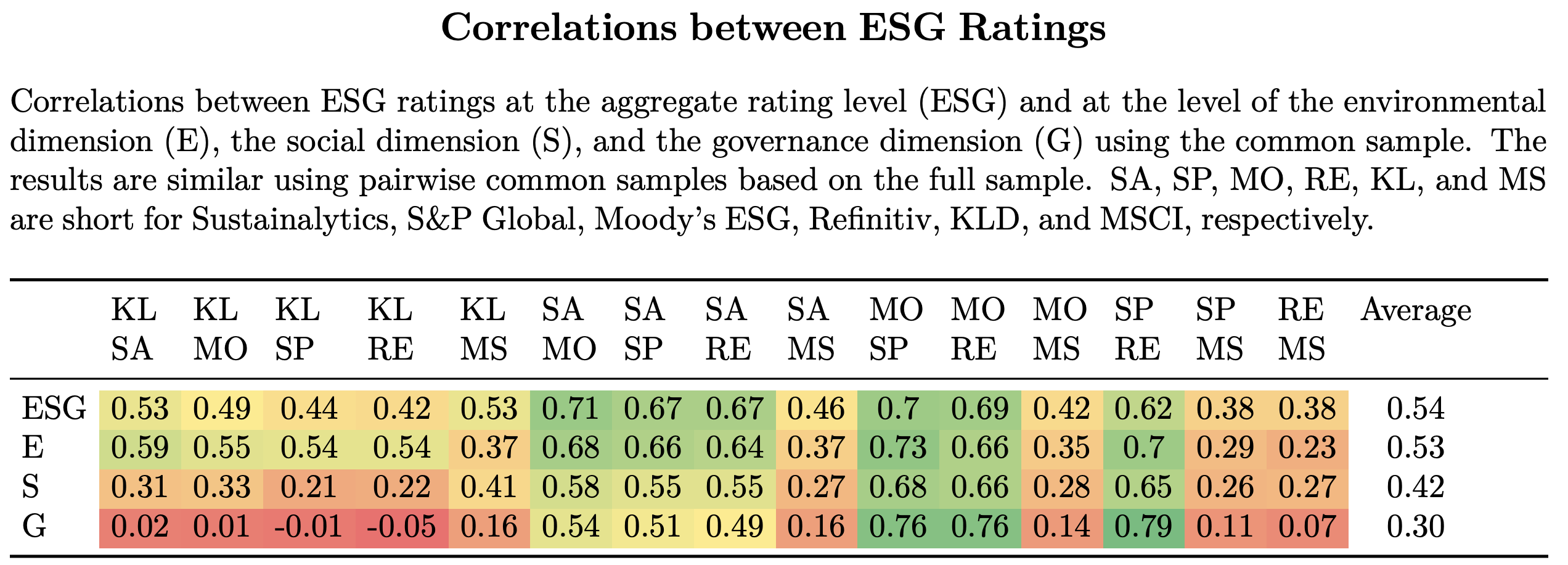
Roughly speaking, a rule of thumb is:
-
strong agreement if correlation above 0.7
-
weak agreement if correlation between 0.3 and 0.7
-
no agreement if correlation between -0.3 and 0.3
-
weak disagreement if correlation between -0.7 and -0.3
- strong disagreement is unlikely…
3.4.4.2 Example of third party (external) evaluation
In a paper in collaboration with Carbon4 Finance, we also document a strong divergence between two raters. One one hand, we have data from a major player, Refinitiv; on the other, we rely on emission scopes computed from Carbon4 Finance methodologies.
For instance, for the airline industry, the evaluation of Scope 3 (downstream) emissions for one given aircraft is:
\[E=C\sum_i U_ie_i,\] where \(U_i\) are the units sold of each type of aircraft and \(e_i\) are induced emissions over the lifetime of the item. The figure is normalized by \(C\), which is the company-specific added-values, measured as the ratio of operating income divided by revenue. The rationale for this scaling is that the firm under consideration is not solely responsible for these downstream emissions. Thus, the responsibility is shared with other entities (e.g., airline companies). The annual emissions of each aircraft \(e_i\) are decomposed as \(e_i=A_iB_iC_iD_iE_i\), where:
- \(A_i\) is the GHG content of jet fuel (tCO2e/L)
- \(B_i\) is the average consumption of aircraft \(i\) (in L/p.km)
- \(C_i\) is the average annual distance traveled (km/year)
- \(D_i\) is the average lifetime of aircraft (years)
- \(E_i\) is the average occupancy (passengers / aircraft).
For the oil and gas sector, the formula is based on the downstream fossil fuel combustion: \[E=\sum_{i,j}V_{i,j}e_{i}v_j,\] where
-
\(i\) is the index of the product type, either liquid (from crude oil to petroleum products, including gasoline, diesel, jet fuel, natural gas liquids (NGLs), heavy fuel oil and others) and gas (conventional, shale, liquefied natural gas (LNG)).
-
\(j\) is the index of the activity carried out along the oil & gas value chain, from upstream (exploration & production) to final energy supply to consumers.
-
\(V_{i,j}\) is the volume of product \(i\) handled in activity \(j\), in tons of oil equivalent (toe).
-
\(e_i\) is the emission factor, i.e., the total amount of CO\(_2\) emissions stemming from the combustion of 1 toe of product type \(i\) (or other non-energy use in the case of petroleum coke).
- \(v_j\) is the value added, approximated here by the ratio of the cost of activity \(j\) divided by the final price paid by the consumer. Again, this scaling reflects the fact that the downstream emissions are not attributable at 100% to the oil or gas extractor.
At the firm-level, we obtain a rather strong divergence between rating providers:
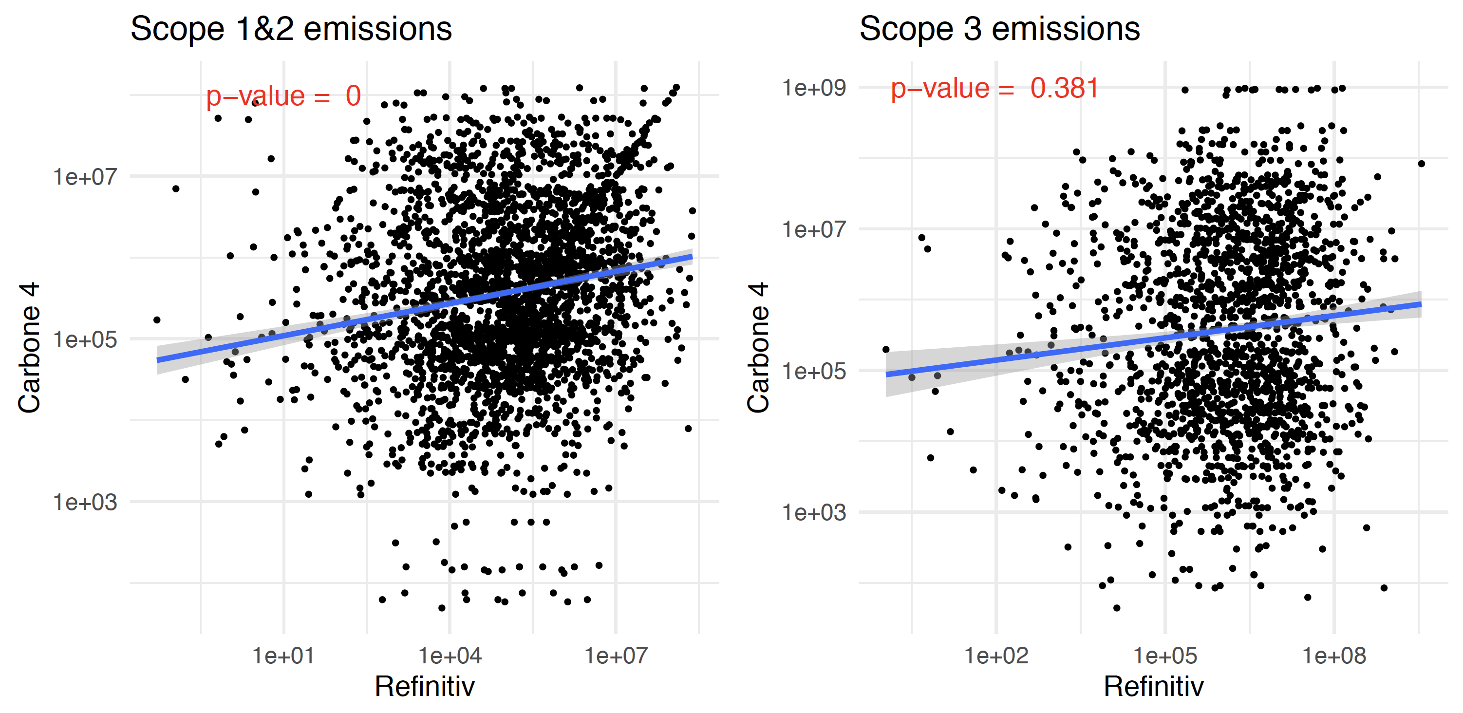
Clearly, scores are all over the place. It is even a bit worse for Scope 3 compared to Scope 1 + Scope 2.
3.4.4.3 In the data?
ESG_data |>
  mutate(year = year(date)) |>
  group_by(source, instrument, year) |>
  summarise(scope_3 = mean(scope_3, na.rm = T)) |>
  pivot_wider(names_from = "source", values_from = "scope_3") |>
  na.omit() |>
  ggplot(aes(x = Provider_A, y = Provider_B, label = instrument)) + geom_point() +
  scale_y_log10() + scale_x_log10() + theme_bw() +
  geom_function(fun = function(x) x, color = "#1199EE") +
  annotate("rect", xmin = 5*10^3, xmax = 10^6, ymin = 0, ymax = 15, alpha = .2) +
  annotate("text", x = 10^5, y = 0.5, label = "Strong disagreement")
The correlation between the two providers is high. The reason?
They probably take most of their numbers from the same source! (corporate reports!)
3.5 Sovereign ESG
3.5.1 Data sources
In contrast with corporate data, sovereign data is much easy to access for free.
There are many organizations that gather and aggregate indicators at the country level, for instance, we can mention:
-
gapminder (independent Swedish foundation). Some fields start in 1800 (deep chronological depth). Great resource if you don’t need too many variables.
-
World Bank: easiest to use from API standpoint (with R, at least).
-
OECD - ok for a few fields, I have not found the API very easy to use.
-
IMF - some features are not available from everywhere!
-
Heritage Foundation: very centered around the notion of “freedom”.
- Institute for Global Environmental Strategies for the Nationally Determined Contributions (NDCs) of countries.
Most of the time, an analyst will need fields from multiple sources, which will require joining datasets… a practice that is very commonplace in data science. Even though some sources (e.g., the World Bank, gapminder) provide exhaustive fields.
Lastly, it is important to mention other sources, like:
- the Carbon monitor initiative. Their aim is to provide almost real-time carbon emissions at a relatively granular level (country). The methodology is outlined in several research papers, from 2020 to late 2022. The updated dataset is available at: https://datas.carbonmonitor.org/API/downloadFullDataset.php?source=carbon_global.
- Germanwatch, and their Climate Change Performance Index (CCPI).
- The ECB: this is news & developing…
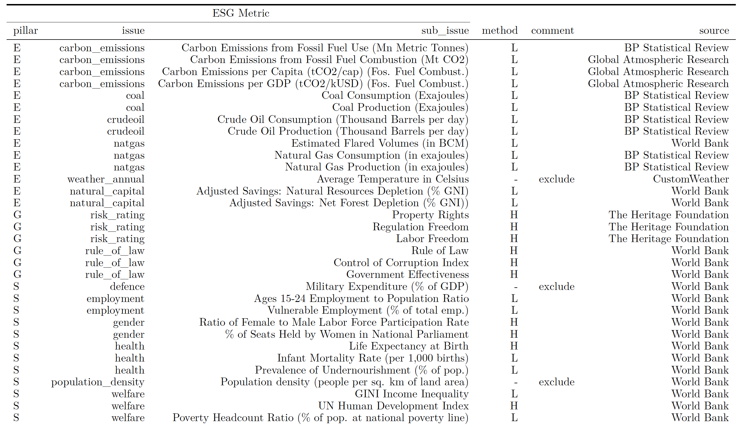
3.5.2 Which pillars?
One example below is taken from the paper Tuning Trend Following Strategies with Macro ESG Data - available upon request.
3.5.3 Geospatial examples
We start with a first example, based on one popular indicator, CO2 emissions (in metric tons per capita).
The data comes from the World Bank: https://data.worldbank.org/indicator/EN.GHG.ALL.PC.CE.AR5.
A list of available indicators is provided here: https://data.worldbank.org/indicator.
The fetching of data will require several packages. Notably, the one, called WDI, that allows to extract data from the World Bank API.
So first, we pull the data and prepare some variables for the map we want to plot.
library(tmap)                         # Geographical plotting
library(countrycode)                  # Package for country codes
library(leaflet)                      # Package for maps
library(sf)                           # Shape files (sf) are a common geographical format
library(WDI)                          # Package that accesses World Bank data

data("World")                         # From tmap!
names(World)[2] <- "country"          # Change the column name
emissions <- WDI(indicator = "EN.GHG.ALL.PC.CE.AR5", start = 2022, end = 2022) |>
  na.omit()                         # Remove missing data
names(emissions)[5] <- "emi_per_cap"  # Change column name

datamap <- World |>
  #mutate(country = country |> recode_factor(`Czech Rep.` = "Czech Republic")) |>
  left_join(emissions |> select(-country), by = c("iso_a3" = "iso3c")) |>
  mutate(emi_per_cap = round(emi_per_cap, 1)) |> # We round numbers
  filter(is.finite(emi_per_cap))
# Below we code the color palette for the map
palet <- colorBin("YlGnBu",                                         # Yellow-Green-Blue palette
                  domain = datamap |> pull(emi_per_cap),            # Domain of labels: emi_per_cap
                  bins = c(0, 1, 2, 5, 10, 15, 80))                 # intervals for CO2 emissions
# Below we code the labels on the map
labels <- sprintf(                                                  # Below we define the labels
  "<strong>%s</strong><br/>%g MtCO2/inhab.",                        # Adding text to label
  datamap$country,                                                  # We show the country name...
  datamap$emi_per_cap                                               # ... and the life expectancy
) |> lapply(htmltools::HTML)                                        # Embedded all into html language
The next chunk of code is one very long call that specifies all the details of the map (no need to look!).
datamap |>
  data.frame() |>                                       # Turn into dataframe (technical)
  sf::st_sf() |>                                        # Format in sf
  st_transform("+init=epsg:4326") |>                    # Convert in particular coordinate reference
  leaflet() |>                                          # Call leaflet
  setView(lng = 0, lat = 20, zoom = 2) |>               # Centering & zooming
  leaflet::addPolygons(fillColor = ~palet(emi_per_cap), # Create the map (colored polygons)
                       weight = 2,                               # Width of separation line
                       opacity = 1,                              # Opacity of separation line
                       color = "white",                          # Color of separation line
                       dashArray = "3",                          # Dash size of separation line
                       fillOpacity = 0.7,                        # Opacity of polygon colors
                       highlight = highlightOptions(             # 5 lines below control the cursor impact
                         weight = 2,                             # Width of line
                         color = "#EEEEEE",                      # Color of line
                         dashArray = "",                         # No dash
                         fillOpacity = 0.9,                      # Opacity
                         bringToFront = TRUE),
                       label = labels,                           # LABEL! Defined above!
                       labelOptions = labelOptions(              # Label options below...
                         style = list("font-weight" = "normal", padding = "3px 8px"),
                         textsize = "15px",
                         direction = "auto")
  ) |>
  leaflet::addLegend(pal = palet,           # Legend: comes from palet colors defined above
                     values = ~emi_per_cap,          # Values come from lifeExp variable
                     opacity = 0.9,                  # Opacity of legend
                     title = "Map Legend",           # Title of legend
                     position = "bottomright")       # Position of legend
Massive discrepancy between Europe and North America.
3.5.4 Time-series analyses
Maps often mostly a static view. It is interesting to have a look at values’ evolution.
We extract other variables below. Several splits thereof are available (male/female, urban/rural).
country_list <- c("AF", "AR", "AU", "BR", "CA", "IN",
                  "CN", "DE", "DZ", "EG", "FR", "GB", # DZ = Algeria
                  "ID", "IR", "JP", "NG", "TR", "US")
wb_data <- WDI(                                             # World Bank data
  indicator = c("ghg_percap" = "EN.GHG.ALL.LU.MT.CE.AR5", # Emissions per capita
                "corrupt_control" = "CC.EST",             # Corruption control
                "life_exp" = "SP.DYN.LE00.IN",            # Life expectancy
                "cpi" = "FP.CPI.TOTL",              # Consumer Price Index (2010=100) = inflation
                "educ_spend" = "SE.XPD.TOTL.GD.ZS", # Government expenditure on education (%GDP)
                "gdp" = "NY.GDP.MKTP.CD",           # Gross Domestic Product (GDP)
                "gdp_growth" = "NY.GDP.MKTP.KD.ZG", # Annual GDP growth
                "pop" = "SP.POP.TOTL"),             # Total population
  country = country_list,                           # Zones: world, US, France, etc.
  start = 2000,
  end = 2022)
This allows us to have a dynamic look of some variables, with geographical focus.
(wb_data |>
   ggplot(aes(x = year, y = educ_spend, color = country)) +
   geom_line() +
   theme_bw() +
   ylab("Education spending")) |> ggplotly()
wb_data |>
  ggplot(aes(x = year, y = gdp_growth, fill = country)) +
  geom_col() +
  facet_wrap(vars(country)) +
  theme_bw() +
  theme(legend.position = "none",
        axis.title.x = element_blank()) +
ylab("GDP growth") 
Some discontinuities in the data: it is far from perfect! No provider is.
3.5.5 Sorting
Ranking is a widely used technique in sustainable finance (more on that later).
Let’s have a look at the corruption control indicator.
wb_data |>
  filter(year == 2020, country != "World", is.finite(corrupt_control)) |>
  mutate(med = median(corrupt_control, na.rm = T),
         corruption = if_else(corrupt_control > med, "High control", "Low control")) |>
  ggplot(aes(x = corrupt_control, y = reorder(country, corrupt_control), fill = corruption)) +
  geom_col() + theme_bw() +
  theme(legend.position = c(0.6,0.3),
        legend.title = element_text(face = "bold"),
        axis.title = element_blank())
3.6 Wrap-up
The key takeaway from this session is that data is one (if not the) cornerstone of sustainable finance.
Measurement accuracy (& availability) is the main issue. Citizens (and investors) want trustworthy data.
Europe seems to be ahead in terms of regulation, but hopefully the US and Asia will follow.
3.7 Exercises
- Pick two (or three) large firms you know or like and try to find ESG related data in one of their annual reports. Can you find common fields, like carbon/GHG emissions?
- With the (excel) dataset from the course, compute carbon intensities (emissions/market cap) with figures from Provider A. With a pivot-table, compute the evolution through time of these intensities. Compare to total emissions. It can typically be the case that total emissions increase while intensities decrease: this would come from the fact that market capitalization grows faster than emissions.